
A Power BI DAX query time comparison of snowflake and star schema based on a sales reporting model done with Power BI.
What
Consider the relationships of the tables in Figure 1 below. The setup is not recommended due to the linking of the dimension/look-up tables of dim_customer and dim_contract. This is a piece of snowflake schema. Figure 2 illustrates a model done with star schema.


For introduction, see for example the following article describing the Power BI star schema basics: https://docs.microsoft.com/en-us/power-bi/guidance/star-schema
Theory
SQLBI has a great article on the costs of relationships: https://www.sqlbi.com/articles/costs-of-relationships-in-dax/. The key message by SQLBI is that large dimension tables are a challenge: ”When you design a star schema, which is the suggested design pattern for this technology, this translates in a bottleneck when you have large dimensions, where large is something that has more than 1-2 million rows. Depending on the hardware, your yellow zone might range between 500,000 and 2,000,000 rows in a dimension. You definitely might expect performance issues with dimensions larger than 10,000,000 rows.”
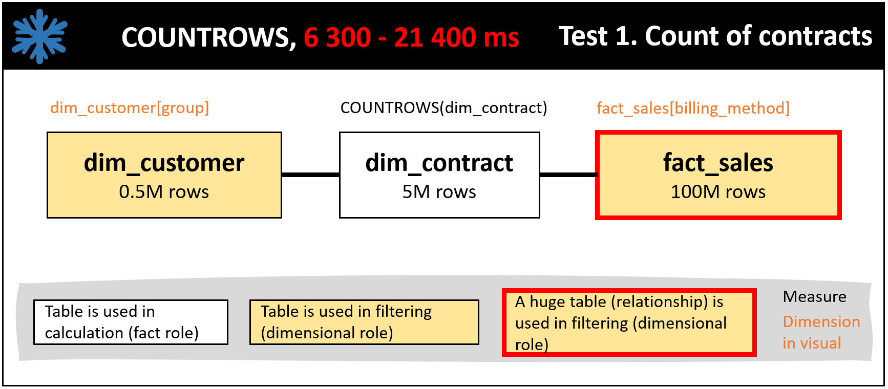
In the DAX query time comparison part of this post, I talk about calculation tables and filter tables. This is due to the fact that in a single DAX measure, it is possible that a dimension table is actually the table which is used for the calculation (e.g. with DAX COUNTROWS function). This can mean that the fact table, or the combination of the fact table and another dimension table, functions as a filter and in a dimensional role.
DAX query time comparison
There are three tests. Test 1 and Test 2 are about counting contracts. Typically, a business wants to follow all kinds of customer and contract counts. Test 3 is about making a customer-level calculation based on two fact tables and pushes the limits of what should be done with a costly DAX measure and large tables.
The benchmarking is done with Power BI built-in Performance Analyzer and Dax Studio with multiple repetitions. The measured value is DAX query time in ms without clearing the cache vs with a cleared cache (e.g. 500 – 1000 ms).
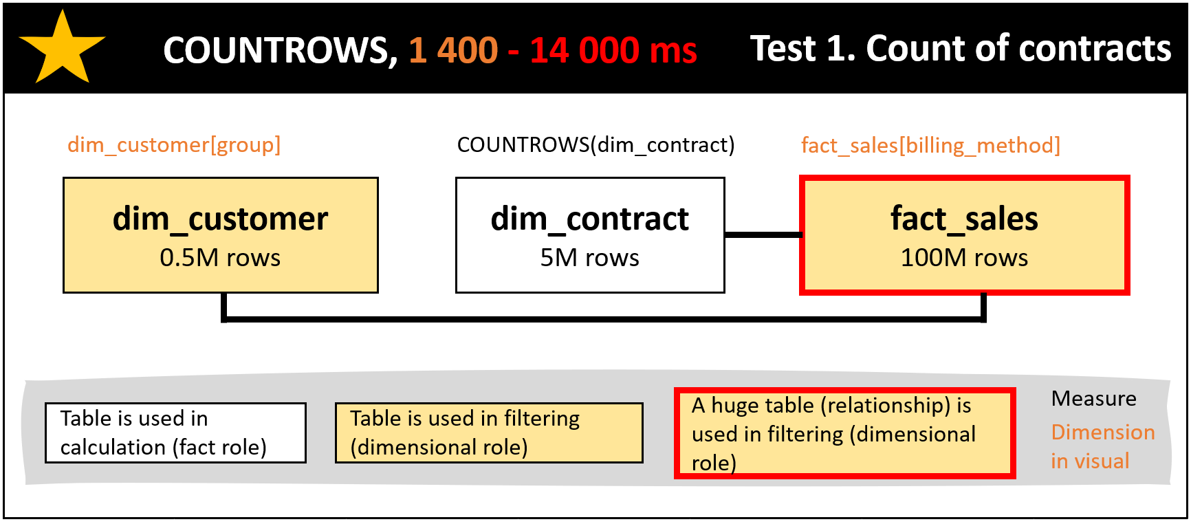
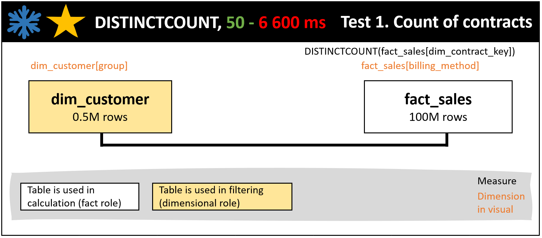
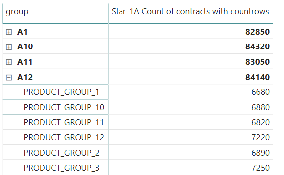
Test 1 is the count of contracts in a stacked column chart with the dimensions of dim_customer[group] and fact_sales[billing_method]. See Figure 3 illustrating the chart. In the comparison are COUNTROWS vs DISTINCTCOUNT functions and snowflake vs star schema. See the results in Figures 4, 5 and 6. The winner is DISTINCTCOUNT (Figure 6) having from the DAX calculation point of view the same schema both with the snowflake and star setup. The Figure 5 setup is faster than the Figure 4 setup thanks to the piece of snowflake in Figure 5 in which dim_customer filters fact_sales making the relationship from fact_sales to dim_contract to have less data.

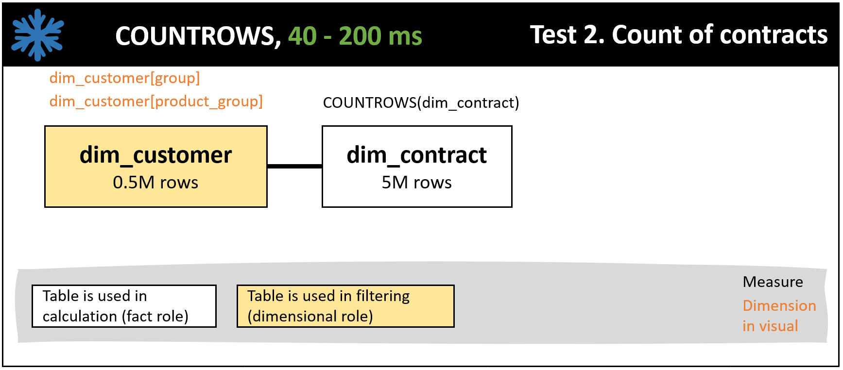
Test 2 is the count of contracts in a matrix table with the dimensions of dim_customer[group] and dim_customer[product_group]. In the test, a drill-down is performed from dim_customer[group] to dim_customer[product_group]. See Figure 7 illustrating the table. The winner is COUNTROWS and snowflake schema (Figure 8) having from the DAX calculation point of view the smallest tables used and the simplest function used.

Test 3 is the iteration of dim_customer rows with SUMX, calculating for each row CALCULATE(MAX(fact_c3[fact_c3_value])*SUM(fact_sales[Value]) and then showing the results as a stacked bar chart with the dimensions of dim_customer[group] and fact_sales[billing_method] like in Figure 3. Here the star schema is the winner (Figure 10) as the snowflake schema (Figure 11) suffers from the use of dim_contract as a bridge table. See my post Power BI DAX How to Calculate in Row Level with Multiple Tables introducing SUMX and how it works in detail.


Code
Here are the used DAX measures.
Star_1A Count of contracts with countrows =
CALCULATE (
    COUNTROWS ( dim_contract );
    KEEPFILTERS ( dim_customer[type] = "snowflake" );
    CROSSFILTER ( fact_sales[dim_customer_key]; dim_customer[dim_customer_key]; BOTH );
    CROSSFILTER ( dim_contract[dim_contract_key]; fact_sales[dim_contract_key]; BOTH );
    USERELATIONSHIP ( fact_sales[dim_customer_key]; dim_customer[dim_customer_key] )
)

Star_1B Count of contracts with distinctcount =
CALCULATE (
    DISTINCTCOUNT ( fact_sales[dim_contract_key] );
    KEEPFILTERS ( dim_customer[type] = "snowflake" );
    CROSSFILTER ( fact_sales[dim_customer_key]; dim_customer[dim_customer_key]; BOTH );
    CROSSFILTER ( dim_contract[dim_contract_key]; fact_sales[dim_contract_key]; BOTH );
    USERELATIONSHIP ( fact_sales[dim_customer_key]; dim_customer[dim_customer_key] )
)

Snowflake_1A Count of contracts with countrows =
CALCULATE (
    COUNTROWS ( dim_contract );
    KEEPFILTERS ( dim_customer[type] = "snowflake" );
    CROSSFILTER ( dim_contract[dim_customer_key]; dim_customer[dim_customer_key]; BOTH );
    CROSSFILTER ( dim_contract[dim_contract_key]; fact_sales[dim_contract_key]; BOTH );
    USERELATIONSHIP ( dim_contract[dim_customer_key]; dim_customer[dim_customer_key] )
)

Snowflake_1B Count of contracts with distinctcount =
CALCULATE (
    DISTINCTCOUNT ( fact_sales[dim_contract_key] );
    KEEPFILTERS ( dim_customer[type] = "snowflake" );
    CROSSFILTER ( dim_contract[dim_customer_key]; dim_customer[dim_customer_key]; BOTH );
    CROSSFILTER ( dim_contract[dim_contract_key]; fact_sales[dim_contract_key]; BOTH );
    USERELATIONSHIP ( dim_contract[dim_customer_key]; dim_customer[dim_customer_key] )
)

Star_3 SUMX fact values =
SUMX (
    dim_customer;
    CALCULATE (
        MAX ( fact_c3[fact_c3_value] )
            * SUM ( fact_sales[sales_value] );
        KEEPFILTERS ( dim_customer[type] = "snowflake" );
        KEEPFILTERS ( fact_sales[dim_calendar_key] = "1" );
        CROSSFILTER ( fact_sales[dim_customer_key]; dim_customer[dim_customer_key]; BOTH );
        CROSSFILTER ( dim_contract[dim_contract_key]; fact_sales[dim_contract_key]; BOTH );
        USERELATIONSHIP ( fact_sales[dim_customer_key]; dim_customer[dim_customer_key] )
    )
)

Snowflake_3 SUMX fact values =
SUMX (
    dim_customer;
    CALCULATE (
        MAX ( fact_c3[fact_c3_value] )
            * SUM ( fact_sales[sales_value] );
        KEEPFILTERS ( dim_customer[type] = "snowflake" );
        KEEPFILTERS ( fact_sales[dim_calendar_key] = "1" );
        CROSSFILTER ( dim_contract[dim_customer_key]; dim_customer[dim_customer_key]; BOTH );
        CROSSFILTER ( dim_contract[dim_contract_key]; fact_sales[dim_contract_key]; BOTH );
        USERELATIONSHIP ( dim_contract[dim_customer_key]; dim_customer[dim_customer_key] )
    )
)
Considerations
Can a table be grouped or aggregated to make the table smaller?
Can some granular dimensions be grouped? Can a fact table be aggregated so that it still answers most business questions? There can be another fact table linked to the data model for selected use cases like the detailed information of a contract or customer. This could be even implemented with Power BI composite models and direct query.
Is it possible to turn fact data into informative dimensions?
Consider a set of fact tables describing sales channel features per order. It might be better to create parameters or segmentation with machine learning which describes how customers behave in different sales channels. This makes the data model less heavy. Same time, business users have a better user experience concentrating on the key facts to improve the business.
One can get rid of a table relationship
One can combine a dimension column with a high cardinality to the fact table to get rid of a costly table relationship. With this decision needs to be checked that all the calculations are logical now and in the future. Combining a dimension to the fact means basically a bidirectional filtering relationship between the fact and the dimension which might not be the desired functionality in some calculations.
Conclusion
It is likely that small changes to a DAX measure, table, or relationship can yield good results compared to building the whole data model again from a scratch. This is clearly visible when the test cases of this post are compared. However, the first time one encounters performance issues actions should be taken. Bad design decisions are likely to repeat making the situation harder to repair. Here are some good links on Power BI and DAX optimization:
https://docs.microsoft.com/en-us/learn/modules/optimize-model-power-bi/
https://maqsoftware.com/expertise/powerbi/power-bi-best-practices
https://maqsoftware.com/expertise/powerbi/dax-best-practices (points 14. and 15. about filtering are really important to use and understand, and give significant performance boost)
https://docs.microsoft.com/en-us/power-bi/guidance/relationships-many-to-many#relate-many-to-many-dimensions
Sample Power BI file
The example measures are created under the customer table in the example file.
https://drive.google.com/file/d/1iuHz2_GGPXj8NpqpCrpjmirb1uRq4xfz/view?usp=sharing